Epicyclificator

Date: 2019-06-15
Author: Diego Plascencia-Vega

Background

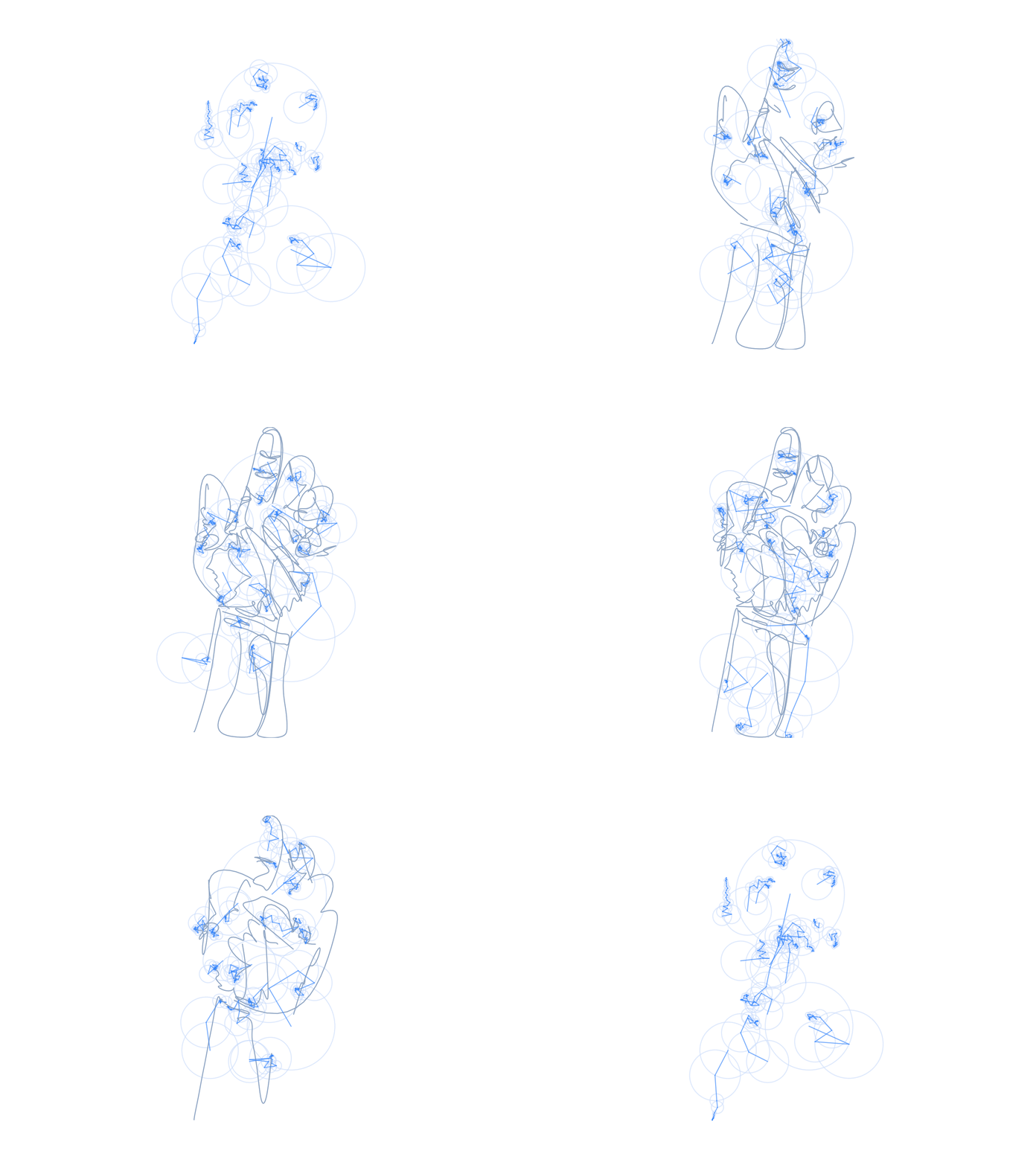
Many articles, blog posts and videos have described the process by which arbitrary closed curve shapes can be approximated by epicycle trajectories. Mathologer [1] walks through an example of how to extract points from a rasterized image and approximate the shape in the image using epicycle trajectories. GoldPlatedGoof [2] walks through a similar process in his video, but starts with a vectorized image in .svg format. Both create these epicycle animations in Mathematica.

In this article I will explain the theory behind how this is done, and show some animations produced by the epicyclificator.

Theory

We can describe motion around a circle using the following equation. \[E(t)=(a+bi)e^{nit}\] Where \((a+bi)\) defines the diameter of the circular motion and where on the circle the cycle starts. \(n\) defines how long it takes the cycle to complete, and which direction the cycle turns.

An epicycle trajecotry can be defined using a series of nested cycles with \(n=-N,...,-1,0,1,...,N\). We will see later why this is a convenient series of \(n\) to choose. The trajectory of the epicycle is defined by the following equation: \[P(t)=\sum_{n=-N}^{N}(a_n+b_ni)e^{nit}=\sum_{n=-N}^{N}C_ne^{nit}\]

To find \(C_n\) we multiply both sides times \(e^{-int}\) resulting in: \[P(t)e^{-nit}=...+C_{n-1}e^{(n-1)it}e^{-nit}+C_ne^{nit}e^{-nit}+C_{n+1}e^{(n+1)it}e^{-nit}+...\] \[P(t)e^{-nit}=...+C_{n-1}e^{-it}+C_n+C_{n+1}e^{it}+...\]

We take the integral of this expression from \(0\) to \(2\pi\). \[\int\limits_0^{2\pi}P(t)e^{-nit}=...+\int\limits_0^{2\pi}C_{n-1}e^{-it}dt+\int\limits_0^{2\pi}C_ndt+\int\limits_0^{2\pi}C_{n+1}e^{it}dt+...\]

For each epicycle, we can use the following property of epicycles: \[\int\limits_0^{2\pi}e^{nit}dt=0\]

Which makes all of the terms on the right zero except for \(C_n\). This simplifies our expression: \[\int\limits_0^{2\pi}P(t)e^{-nit}=C_n2\pi\] \[\frac{1}{2\pi}\int\limits_0^{2\pi}P(t)e^{-nit}=C_n\]

We can use the above expression to find all \(C_n\) terms that make up the epicycle approximating the closed curve of interest.